AWS Certification

I have been recently working on my AWS Certification. I am trying to take as many positives as I can with the lockdown situation at the moment. It’s been a busy month studying and more importantly, spend time on labs and practising for my AWS exam. Now I’m a proud holder of AWS Cloud Practitioner Certificate.

Pandas in a Nutshell

Hi,

Hope you enjoyed my previous article and introduction to NumPy .

The purpose of today’s blog post is to follow the same format but go through some pandas topics. Pandas is an open source library built on top of numpy. It provides easy to use data structures for data analysis, time series and statistics. Pandas is like Python’s version of Excel or R. Let’s get started.

Series is similar to the numpy array but pandas series can be label indexed. On the same note, another main difference between pandas series and numpy array is that pandas series can have objects of different types.

You can use a Python list, numpy array or even a dictionary to create a Series. See below an example which creates series from numpy array.

 

The index is a key thing with the Series allowing quick lookup access of the data. I will use the top headline of the Coronavirus at the moment as an example. In this case, the label is the country with data points against it.

 

Moving on to the next topic which is dataframes. Think of a dataframe as a bunch of series sharing the index. In the example below, df uses the default labels of 0, 1 and 2 with some values for columns X, Y and Z. df_rand has been created from random values and has both labels and column headers named accordingly. X, Y, Z column is a Series itself. You can also read a dataframe from a csv file.

 

Now let’s just select a row which would be a Series too. If more than one row is selected, then obviously that’s a dataframe 🙂

 

Similarly to numpy, pandas have the ability to apply conditional selection.

 

Finally, let’s demonstrate how to join dataframes together or ultimately stack them. If you have SQL background,  then this should be easy peasy.

Enjoy! 🙂

 

NumPy in a Nutshell

Hello and welcome back. I have started a new category in my blog about Python. The purpose of this post is to go through NumPy library. I will be using Jupyter for the demo but will provide the py file if you prefer to run it in PyCharm for example. NumPy is a core Python Linear Algebra library for Data Science used for faster array processing than the native Python lists with a bunch of handy methods. Let’s make a start!

 

You can cast a normal list to a one-dimensional array using the array function.

Or have a list of list and cast it as a two-dimensional array. This effectively is a matrix that has 2 rows and 4 columns. The size attribute gives the number of elements of the array.

Next section shows different ways to create NumPy arrays.

Functions ones and zeros are a handy way to create arrays of 1s and 0s. Linspace is another function similar to arange but using equal steps. Also check out reshape and ravel().

See examples of other useful methods below.

Next, let’s have a look at selections and indexing.

Great stuff. To Illustrate the indexing, let’s create a new two-dimensional array.

Let’s see what other operations you can do apart from copy().

Let’s have a look at some basic operations like += or *= to change an existing array instead of creating a new one. Check out how to calculate the sum of all elements of an array or find the min or max value below.

As promised see below the py file with all the examples.

import numpy as np

# normal list
v_even_list = [20, 40, 60]

print(v_even_list)

# cast to 1-dimensional array

print(np.array(v_even_list))

# 2-dimensional array

v_matrix = np.array([[10,20,30,40],
                     [50, 60, 70, 80]])

print(v_matrix)

print(v_matrix.shape)

print(v_matrix.size)




# Create Array:

# Use arange

v_array = np.arange(20)


print(v_array)


# Use array to create one-dimensional array


v_array1 = np.array([1,3,5])


print(v_array1)


# Use array to create n-dimensional array


v_array2 = np.array([[1,2,3],
                     [4,5,6],
                     [7,8,9],
                     [10,11,12]])



print(v_array2)


v_array3 = np.array([(2.25,3.25,4.25), (5,6,7)])



print(v_array3)


# Create array of 1s. Note default type is float64

v_one = np.ones((2,3))

print(v_one)


# Create array of 0s, specify the type needed


v_zero = np.zeros((2,4), dtype=np.int16)



print(v_zero)


# Array of 3 numbers between 5 and 10 in equal steps


v_eq_steps = np.linspace(5,10, 3)



print(v_eq_steps)


# 2-dimensional array with 3 rows and 5 columns to modify the shape the way you need.
# ravel() is the opposite and will flatten the array


r = np.arange(15).reshape(3,5)

print(r)

# Array of random values in this case a matrix with 2 rows and 3 columns

v_array = np.random.rand(2,3)


print(v_array)

# Random 20 integer values in the range of 10 and 100

v_arr_int = np.random.randint(10, 100, 20)


print(v_arr_int)


# The index of the min value in the array

print(v_arr_int.argmin())


# The index of the max value in the array

print(v_arr_int.argmax())


# return elements of the array where value is > 30


print(v_arr_int[v_arr_int>30])




# Create a sample array


v_array = np.arange(20)


print(v_array)


# Slice from index 5 to 10


print(v_array[5:10])


# Everything up to index 10

print(v_array[:10])


# All elements beyond index 10


print(v_array[10:])


# We can assign values which is called broadcast and then slice


v_array[15:20]=-5


print(v_array)

v_slice_array = v_array[15:20]


print(v_slice_array)


# Broadcast actually change the original array.
# You can use v_array.copy() to keep the original values

# Create a sample matrix



v_matrix = np.array([[1,2,3,4],
                    [5,6,7,8]])


print(v_matrix)


# Get the row specified by the index

print(v_matrix[0])


# Get just one value - the element from the last row and last column

print(v_matrix[1,3])



# Return submatrices eg a slice which is anything beyond row 0 and after column 2


print(v_matrix[0:,2:])


# Nice one!


# Create a sample with 0s

# In[2]:


m = np.zeros((2,4), dtype = int)


print(m)


# Modify existing a to add 5

m += 5

print(m)


# Modify a to multiply by 4

m *= 4


print(m)

print(m.sum())


print(m.min())


print(m.max())


# Sum of each column

print(m.sum(axis = 0))


# Cumulative sum of each row

b = np.arange(6).reshape(2,3)

print(b)

print(b.cumsum(axis = 1))

 

That’s all for now. Stay tuned.

 

Cheers,

Maria

Ingesting data into Hive using Spark

Before heading off for my hols at the end of this week to soak up some sun with my gorgeous princess, I thought I would write another blog post. Two posts in a row – that has not happened for ages 🙂

 

My previous post was about loading a text file into Hadoop using Hive. Today what I am looking to do is to load the same file into a Hive table but using Spark this time.

I like it when you have options to choose from and use the most appropriate technology that will best fit into customers requirements and needs with respect to technical architecture and design. You obviously need to bare in mind performance as always!

You would usually consider using Spark when the requirements call for fast interactive processing. Conversely, in the case of batch processing, you would go for Hive or Pig. So going back to Apache Spark, it is a powerful engine for large-scale in-memory data processing and this is where Spark fits against all data access tools in the Hadoop ecosystem.

In a nutshell, Spark is fast and runs programs up to x100 faster than MapReduce jobs in memory, or x10 faster on disk. You can use it from Scala, Python and R shells.

I am not going into much more details here, but just a quick intro though to flesh out the concepts so that we all stay on the same page.  Spark’s data abstractions are:

• RDD – resilient distributed dataset eg RDDs can be created from HDFS files
• DataFrame – built on top of RDD or created from Hive tables or external SQL/NoSQL databases. Similar to the RDBMS world, data is organized into columns

 

Alright, let’s get started. Butterflies in my stomach again.

I will use PySpark – Spark via Python as you can guess.

[maria_dev@sandbox ~]$ pyspark

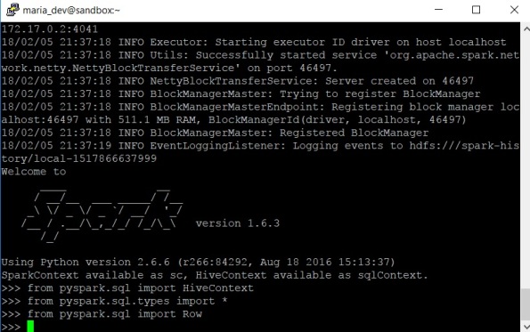
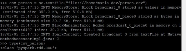
1. First import the local raw csv file into a Spark RDD

>>> csv_person = sc.textFile(“file:///home/maria_dev/person.csv”)

>>> type(csv_person)

By using the type command above, you can quickly double check the import into the RDD is successful.

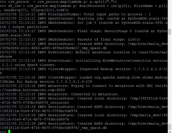
2. Use Spark’s map( ) function to split csv data into a new csv_person RDD

>>> csv_person = csv_person.map(lambda p: p.split(“,”))

3. Use toDF() function to put the data from the new RDD into a Spark DataFrame

Notice the use of the map() function to associate each RDD item with a row object in the DataFrame. Row() captures the mapping of the single values into named columns in a row to be saved into the new DataFrame.

>>> df_csv = csv_person.map(lambda p: Row(PersonId = int(p[0]), FirstName = p[1], Gender=p[2], City=p[3])).toDF()

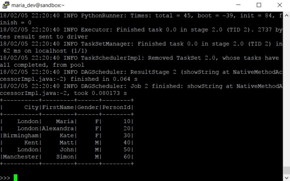
4. Verify all 6 rows of data in df_csv DataFrame with show command

>>> df_csv.show(6)

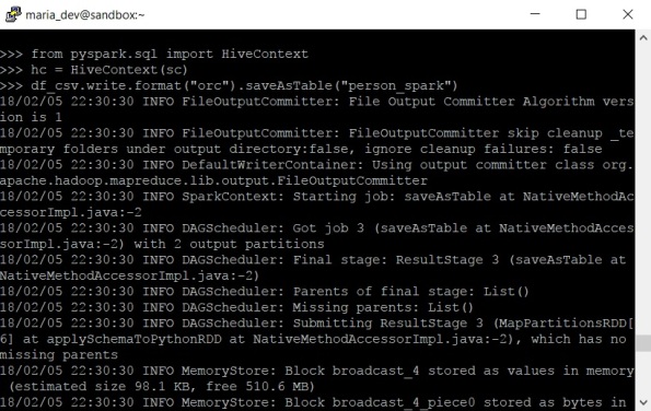
5. Finally, use saveAsTable() to store the data from the DataFrame into a Hive table in ORC format

>>> from pyspark.sql import HiveContext
>>> hc = HiveContext(sc)
>>> df_csv.write.format(“orc”).saveAsTable(“person_spark”)

6. Log in Ambari Hive to check your table

 

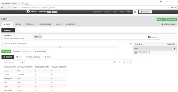
There you go. Happy days 🙂

 

Cheers,

Maria

 

Loading data in Hadoop with Hive

It’s been a busy month but 2018 begins with a new post.

 

A common Big Data scenario is to use Hadoop for transforming data and data ingestion – in other words using Hadoop for ETL.

In this post, I will show an example of how to load a comma separated values text file into HDFS. Once the file is moved in HDFS, use Apache Hive to create a table and load the data into a Hive warehouse. In this case Hive is used as an ETL tool so to speak. Once the data is loaded, it can be analysed with SQL queries in Hive. Then data is available to be provisioned to any BI tool that supports Hadoop Hive connectors like Qlik or Tableau. You can even connect Excel to Hadoop by using Microsoft Power Query for Excel add-in. Exciting, isn’t it !?!

Well, let’s get started.

 

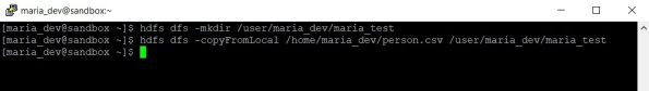
1. Move file into HDFS

First, create an input directory in HDFS and copy the file from the local file system.

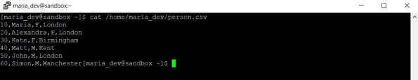
I have created a sample person.csv file where the first two records are myself and my lovely daughter Alexandra. Who knows she may teach me some supa dupa technologies one day, though she is more into art and dance for now 🙂

10,Maria,F,London

20,Alexandra,F,London

30,Kate,F,Birmingham

40,Matt,M,Kent

50,John,M,London

[maria_dev@sandbox ~]$ hdfs dfs -mkdir /user/maria_dev/maria_test

[maria_dev@sandbox ~]$ hdfs dfs -copyFromLocal /home/maria_dev/person.csv /user/maria_dev/maria_test

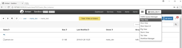
For the purposes of this demo I will use Hortonworks sandbox. If you now log in Ambari and navigate to Files View, you should be able to see the file just copied into HDFS.

2. Create an external table

Very quickly here, Hive supports two types of tables:

• Internal – it is managed by Hive and if deleted both the definition and data will be deleted
• External – as the name suggests, it is not managed by Hive and if deleted only the metadata is deleted but the data remains

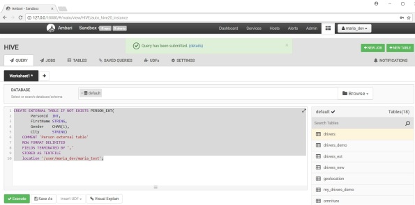
Run the command below either from Hive command line or Hive View in Ambari. I use Ambari.

CREATE EXTERNAL TABLE IF NOT EXISTS PERSON_EXT(

PersonId INT,

FirstName STRING,

Gender CHAR(1),

City STRING)

COMMENT ‘Person external table’

ROW FORMAT DELIMITED

FIELDS TERMINATED BY ‘,’

STORED AS TEXTFILE

location ‘/user/maria_dev/maria_test’;

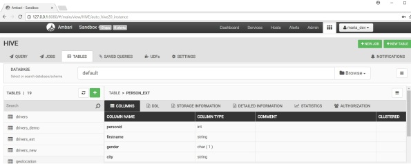
You can find the external table now in the list of tables.

Verify the import is successful by querying the data with HSQL.

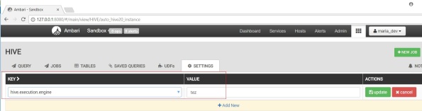
Before moving to the next step, let me quickly mention Tez engine here. Tez has some great improvements in terms of performance of the Hive queries in comparison with the standard MapReduce execution engine. To get speed improvements, make sure you have Tez enabled which is done via the Hive View Settings tab as show below.

3. Create internal table stored as ORC

ORC is an optimized row columnar format that significantly improves Hive performance. There are other formats that can be used such as sequence or text file but ORC and Parquet are most commonly used mainly because of the performance and compression benefits.

Run the create command below.

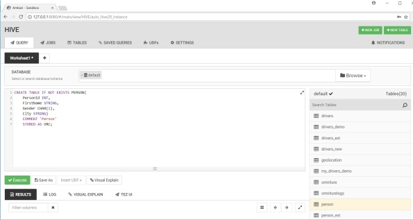
CREATE TABLE IF NOT EXISTS PERSON(

PersonId INT,

FirstName STRING,

Gender CHAR(1),

City STRING)

COMMENT ‘Person’

STORED AS ORC;

After successfully ran the command you will see person table on the right.

So far so good. It is time now to load the actual data.

4. Copy data from the external table into the internal Hive table

Use INSERT SELECT to load the data.

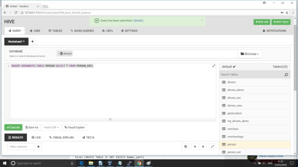
Verify data has been successfully loaded.

 

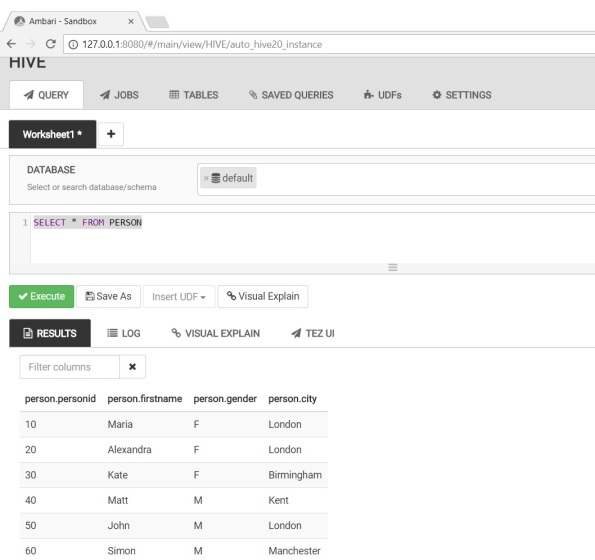
Fab, good stuff – nice and simple.

Hope you enjoyed this!

 

Cheers,

Maria

 

 

Big Data Marathon

This week there is a Big Data event in London, gathering Big Data clients, geeks and vendors from all over to speak on the latest trends, projects, platforms and products which helps everyone to stay on the same page and align the steering wheel as well as get a feeling of where the fast-pacing technology world is going. The event is massive but I am glad I could make it even only for one hour and have some fruitful chats with the exhibitors. The ones which are of particular interest to me are Cloudera, Hortonworks, Informatica with Big Data Management and ICS, MapR, Datalytyx. Check here for more information https://bigdataldn.com/

 

Nowadays, with the massive explosion of data in the digital era we all live in, it is not difficult to notice the evolution of Data to Big Data. With the new sources of data, the variety of data has changed – unstructured(text, images, videos), semi-structured(JSON, facebook graphs) and structured. Big Data drives asking new questions which require the use of predictive, behavioural models and machine learning. In a nut shell, in terms of physical storage the options are Cloud or on premise and in terms of logical storage – RDBMS, Hadoop, NoSQL.

 

The use of Hadoop may include the use of libraries that layer NoSQL implementations on top of HDFS data. Hadoop is a datastore or a data lake for a lot of customers and is a replacement in some way of a relational database. On this point here, I would like to stress out that RDBMS like Oracle are still around and they are not going to disappear from the Big Data picture as they are designed to solve specific set of data problems that Hadoop is not designed to solve. Having said that, bringing in Hadoop as a solution will be as an addition to existing RDBMS and not a replacement of customers’ EDW.

 

Cheers,

Maria

How to Install and Configure OBIEE 12c

Oracle BI 12c has been released for some time now. There are a few changes in the way it is installed compared to the previous 11g releases. This post is about installing and configuring OBIEE 12c with detailed step-by-step instructions(Linux x86-64 in this case).

 

You can start with downloading the media from OTN :

1. Download and install JDK8(at least 1.8.0_40)

2. Download and install Weblogic Server

fmw_12.2.1.0.0_infrastructure_Disk1_1of1.zip

3. Download and install Oracle Business Intelligence 12c (12.2.1.0.0)

fmw_12.2.1.0.0_bi_linux64_Disk1_1of2.zip

fmw_12.2.1.0.0_bi_linux64_Disk1_2of2.zip

 

Now let’s start with the steps above.

1. After JDK8 is installed export environment variables and add this to the profile if needed.

export JAVA_HOME=/usr/java/jdk1.8.0_65

export PATH=$JAVA_HOME/bin:$PATH

 

2. Install Oracle Fusion Middleware Infrastructure

$ unzip -q fmw_12.2.1.0.0_infrastructure_Disk1_1of1.zip
$ $JAVA_HOME/bin/java -d64 -jar fmw_12.2.1.0.0_infrastructure.jar

 

 

Click Next to continue and then choose ‘Skip Auto Updates’ and then click Next.

 

 

Choose the Fusion Middleware Home location for example /app/oracle/obiee12c

 

 

Choose Fusion Middleware Infrastructure with Examples in case you are keen on playing with them.

 

 

Click Next after all system configuration checks are successful.

 

 

Choose Next and continue to next screen.

 

 

Choose Install to proceed with the installation.

 

 

Click Finish to complete the installation.

 

 

Oracle Fusion Middleware Infrastructure 12c is now installed.

 

3. Install OBIEE

To begin with OPMN is no more used in Oracle Fusion Middleware and is deprecated in 12c. You can check more about OBIEE 12c New Features here.

Navigate to the directory where you downloaded the media and unzip the two files.

$ cd /home/oracle/obiee12c

$ unzip -q fmw_12.2.1.0.0_bi_linux64_Disk1_1of2.zip

$ unzip -q fmw_12.2.1.0.0_bi_linux64_Disk1_2of2.zip

$ ./bi_platform-12.2.1.0.0_linux64.bin

 

Choose Next

 

 

 

Again choose Skip Auto Updates and then click Next.

 

 

Specify the same Fusion Middleware home from the steps above.

 

 

Choose BI Platform with Samples in case you want to play with the Sample Apps.

 

 

When all system configuration checks are passed click Next.

 

 

Choose Install to proceed with the installation.

 

 

Choose Finish to complete the installation.

 

 

OBIEE 12c is now installed. Next part of this post will cover the repository creation.

 

4. Repository creation

The RCU – Repository Creation Utility is no more a separate download as it used to be in the previous releases. It is now part of the software installation. You can start RCU as shown below:

$ cd /app/oracle/obiee12c/oracle_common/bin

$ ./rcu

 

 

 

Click Next and then choose Create Repository and then System Load and Product Load if you have DBA privileges.

 

 

Specify the Oracle database details. Note that Oracle Fusion Middleware 12c requires Oracle Database 11g R2(11.2.0.4) or higher. Bare in mind if you go with Oracle 12c you’d better use a container database as non-container architecture is deprecated in Oracle Database 12c, and may be desupported and unavailable in a release after Oracle Database 12cRelease 2. Oracle recommendation is to use the container architecture.

 

 

Click OK when prerequisite checks are completed and choose Next.

 

 

Choose the prefix for the schemas to be created, in this case the default DEV.

 

 

Click OK when prerequisite checks are completed and choose Next.

 

 

Provide password(s) for the schemas to be created.

 

 

Choose Next

 

 

Click OK

 

 

Click Create to confirm the schemas which will be created.

 

 

Click Close to exit from RCU. With this step the repositories creation is complete.

 

 

Next section will cover the configuration of OBIEE 12c.

 

5. Configure OBIEE 12c

 

Navigate to <OBIEE_HOME>/bi/bin and start the configuration utility script.

 

$ cd /app/oracle/obiee12c/bi/bin
$ ./config.sh

 

 

 

Select components to install in this case just Business Intelligence Enterprise Edition and then click Next.

 

 

Click Next when all system checks are completed.

 

 

Specify the details for the BI domain to be created.

 

 

The repositories schemas are created with the RCU so choose Use existing schemas to continue. You have the option to create the schemas at this step too if you haven’t done this yet.

 

 

 

Specify the port numbers in this case default values.

 

 

Choose SampleAppLite in case you need this.

 

 

On the next screen click Configure. This step will take a while to get the configuration completed.

 

 

Click Next and you will get the configuration complete screen.

 

 

It is always useful to save the configuration install log file. Click Finish to complete the configuration.

 

 

Once this is done a browser window opens up automatically for you to login to OBIEE.

 

 

 

 

This post will end up with listing the basic commands to manage the services. The scripts for this are located in <OBIEE_HOME>/user_projects/domains/bi/bitools/bin

• start.sh
• status.sh
• stop.sh

Hello OBIEE 12c world. Enjoy!

BGOUG 2015 Autumn Conference

The autumn BGOUG conference is now over. I planned to write a post immediately after the end of the conference when the enthusiasm and spirit is still fresh bee-zing but anyway it stays for quite a while  🙂

This year it was the whole family attending the conference and my daughter Alex had an early Oracle start listening to Jonathan Lewis talking about execution plans.

This time we had about 370 people attending BGOUG. My presentation on Three Sides of the Coin with Oracle Data Integration – ODI, OGG, EDQ went very well and I had a full room of people. I also had a live 30 minutes demo which went smoothly and I managed to fit to the 60 mins all together. I attended Jonathan Lewis’s, Joze Senegacnik’s , Gurcan Orhan’s sessions. Not as many as I initially thought. I planned to listen Heli, Julian Dontcheff and Martin Widlake at least but I couldn’t do it. I am sure I will see Martin at the LOB events in London anyway.

It was really nice to catch up with old friends and colleagues and also make new friends. I am glad I met Osama Mustafa and Joel Goodman in person. I haven’t seen Julian for quite a while and it was a real pleasure to see him again and meet his Accenture colleagues. Same for Joze and Lili. Obviously BGOUG is like a big family(without the fights) and it is quite an international one.

Big thanks to Milena for organizing this great event. The whole team has been doing great job for  all these years now. Really nice idea to start printing the number of visits and tracking this for each attendee. I have now 16 and Joze has 14 and I have to be very careful with that 🙂

 

All in all, it was a great event, presentations, great people, very nice venue, hotel, food, party till midnight. I would say keep up the good work!

 

Cheers,

Maria

 

 

ODI 12c 12.1.3 oci driver

When you connect from ODI Studio 12c to the repository you may get error “no ocijdbc in java.library.path”. In my case I use ODI Studio 12c installed on Windows 7 64bit machine and connecting to ODI 12c linux environment. So why do I get this error?

 

 

On the same note I use Oracle JDBC Driver ODI driver connection. As the studio does not use the tnsnames to connect to the Oracle instance if you try jdbc:oracle:oci8:@<tns_alias> it will not work. That’s why you can give (DESCRIPTION=(ADDRESS=(PROTOCOL=TCP)(HOST=hostname)(PORT=1521))(CONNECT_DATA=(SERVER=DEDICATED)(SERVICE_NAME=SID))) instead. So far so good but still get the same error.

 

This error gives me a signal it might be because of incompatibility of the jdbc drivers coming with ODI 12c and the Oracle client. As a starting point I have Oracle 11.2.0.4 client installed on my station. Let’s check what version ODI 12c uses, probably 12? Check this in <<ODI_HOME>>\oracle_common\modules\oracle.jdbc_12.1.0\ojdbc6dms\META-INF\MANIFEST.MF

 

Implementation-Version: 12.1.0.2.0

 

Now it makes perfect sense. Let’s install Oracle 12.1.0.2.0 client. Once this is done two more things needed. Add the following line in <<ODI_HOME>>\odi\studio\bin\odi.conf\odi.conf

 

AddVMOption -Djava.library.path=<<ORACLE_HOME>>\bin

 

The second thing is to set the system variables for

ORACLE_HOME=C:\Oracle\client12c

LD_LIBRARY_PATH=%ORACLE_HOME%\lib value

PATH=%ORACLE_HOME%\bin;%PATH% value

 

Enjoy ODI 12c world!  

 

Cheers,

Maria

New beginning

Happy New Year everyone. I wish you a prosperous 2015!

Time is passing by too fast. I had a dynamic 2014 with a couple of interesting projects. It’s not time to recap now but it is definitely time to refresh my blog.

For me with the new year comes the new beginning too. I switched from contracting to permanent job because I’ve always wanted to work for an Oracle partner in the UK with big Oracle projects. I am very pleased I joined Peak Indicators as a BI Consultant to work on OBIEE and ODI projects. Peak Indicators is an experienced Business Intelligence consulting company which is an Oracle Gold Partner highly specialized in Oracle Business Intelligence.

I had a trip to Chesterfield to meet the colleagues there and some in London. I am glad that a week after I started I had the chance to install OBIEE and apply latest OBIEE bundle patch (11.1.1.7.150120)  released this Tuesday. So I started to get the feel of it and I would say there is a lot to crunch. I hope I will be able to blog more and attend UKOUG as well as BGOUG.

 

Cheers,

Maria